Matt Dray
⚠️ Warning: this post contains offensive words. ⚠️

Genius?
Kanye West released his latest album – ye – last week1 after a(nother) pretty turbulent and controversial period of his life2. So what’s been on his mind?
I think the real question is why don’t we scrape Yeezus’s lyrics from the web and analyse them using R? Obviously.
Genius
Genius is a website where you can upload and comment on song lyrics. It’s like Pop Up Video for young people.
You can access the lyrics data via Genius’s API3. Luckily, the R package genuisr was developed by Ewen Henderson for exactly this purpose.4
Access the API
You need to register with Genius so you can get tokens for accessing their API. To do this:
- Create a new Genius API client.
- Click ‘generate access token’ under ‘client access token’ to generate an access token.
- After
install.packages("geniusr"),library(geniusr)you’ll be prompted to enter the access token when you try to use ageniusrfunction
I stored the token in my .Renviron file. This is a file for store variables that R will look for and load automatically on startup. Edit the file on your system by running usethis::edit_r_environ() and adding the line GENIUS_API_TOKEN=X, replacing X with your token.
If you don’t store your token this way then you’ll be prompted for a new token every time you start a new R session, which could get quite tedious. It also means you don’t have to store it in plain sight
Use geniusr
Find Kanye
First we need to find the artist ID for Kanye. We can use search_artist() to look for him.
library(geniusr)  # access genius api
library(dplyr)  # manipulate data
library(knitr)  # pretty table printing

geniusr::search_artist("kanye west") %>%
knitr::kable() # prints the table nice| artist_id | artist_name | artist_url |
|---|---|---|
| 72 | Kanye West | https://genius.com/artists/Kanye-west |
| 652275 | JAY-Z & Kanye West | https://genius.com/artists/Jay-z-and-kanye-west |
Kanye’s ID on Genius is 72 as a solo artist. We can save this value as the object kanye_id and use it to get metadata about him. This includes the web address for his artist page on Genius, a link to the image of him used on the site and the number of people ‘following’ his lyrics page.
# artist ID
kanye_id <- 72

# access meta info
artist_meta <- geniusr::get_artist_meta(
  artist_id = kanye_id
)

# preview
dplyr::glimpse(artist_meta)
## Observations: 1
## Variables: 5
## $ artist_id <int> 72
## $ artist_name <chr> "Kanye West"
## $ artist_url <chr> "https://genius.com/artists/Kanye-west"
## $ artist_image_url <chr> "https://images.genius.com/92fee84306e9a1ec88...
## $ followers_count <int> 8754Get songs
Now we can use Kanye’s artist ID to obtain all his songs on Genius.
# get all songs for a given artist id
kanye_songs <- geniusr::get_artist_songs(
  artist_id = kanye_id
)

# a random preview
dplyr::sample_n(kanye_songs, 10) %>%
  dplyr::select(song_name) %>%
knitr::kable()| song_name |
|---|
| Can’t Tell Me Nothing (Official Remix) (Ft. Jeezy) |
| On Meeting with Donald Trump |
| Last Call |
| Oh Oh |
| See You In My Nightmares (Live From VH1 Storytellers) |
| Paranoid (Ft. Mr. Hudson) |
| Father Stretch My Hands Pt. 1 (Ft. Kid Cudi) |
| Late |
| Unreleaased Studio Session |
| Porno (Interlude) |
We can also access a greater list of data for each song, including the album name and release date. We can use the map_df function from the purrr package to look for the meta data for each song in turn.
library(purrr)  # functional programming

# apply function over each song id
songs_meta <- purrr::map_df(
  kanye_songs$song_id,
  geniusr::get_song_meta
)

# a random preview
dplyr::sample_n(songs_meta, 10) %>%
  dplyr::select(song_name, album_name) %>%
knitr::kable()| song_name | album_name |
|---|---|
| Never See Me Again | NA |
| Olskoolicegre | I’m Good |
| Just Soprano Freestyle | NA |
| BET Cypher 2010 (Kanye West, Big Sean, Pusha T, & Common) (Ft. Big Sean, Common, CyHi The Prynce & Pusha-T) | NA |
| Blue Note NYC Freestyle (2nd Verse) | NA |
| Electric Relaxation 2003 (Ft. Consequence) | I’m Good |
| Magic Man (Ft. Malik Yusef) | NA |
| Two Words (9th Wonder remix) | NA |
| Drive Slow (A-Trak remix) (Ft. GLC & Paul Wall) | NA |
| Clique Freestyle | NA |
Looking at the album names, it seems we’ve got songs from 37 albums at least plus a bunch that are unknown or unclassified.
# the songs are from which albums?
unique(songs_meta$album_name)
## [1] NA
## [2] "Def Poetry Jam"
## [3] "Kanye West's Visionary Streams of Consciousness"
## [4] "Zane Lowe BBC Radio Interviews (Kanye West)"
## [5] "The Life of Pablo"
## [6] "808s & Heartbreak"
## [7] "Late Registration"
## [8] "The College Dropout"
## [9] "Freshmen Adjustment"
## [10] "World Record Holders"
## [11] "ye"
## [12] "My Beautiful Dark Twisted Fantasy"
## [13] "VH1 Storytellers"
## [14] "Get Well Soon..."
## [15] "Freshmen Adjustment Vol. 2"
## [16] "The Cons, Volume 5: Refuse to Die"
## [17] "Graduation"
## [18] "Can't Tell Me Nothing"
## [19] "Kon the Louis Vuitton Don"
## [20] "Yeezus"
## [21] "I'm Good"
## [22] "Graduation \"Bonus Tracks, Remixes, Unreleased\" EP"
## [23] "Turbo Grafx 16*"
## [24] "G.O.O.D. Fridays"
## [25] "Kanye West Presents Good Music Cruel Summer"
## [26] "Kanye's Poop-di-Scoopty 2018"
## [27] "King"
## [28] "Freshmen Adjustment Vol. 3"
## [29] "2016 G.O.O.D. Fridays"
## [30] "Welcome to Kanye's Soul Mix Show"
## [31] "Late Orchestration"
## [32] "College Dropout: Video Anthology"
## [33] "The Lost Tapes"
## [34] "NBA 2K13 Soundtrack"
## [35] "Rapper's Delight"
## [36] "Boys Don't Cry (Magazine)"
## [37] "The Man With the Iron Fists (Original Motion Picture Soundtrack)"
## [38] "Coach Carter (Music from the Motion Picture)"So you can see ye is definitely in the list of albums and we can filter our data frame so we just get the seven tracks from that particular album. Maybe we’ll explore the other lyrics more deeply another day.
# filter songs from album 'ye'
ye <- songs_meta %>%
  dplyr::filter(album_name == "ye")

# preview songs
dplyr::select(ye, song_name)
## # A tibble: 7 x 1
## song_name
## <chr>
## 1 All Mine
## 2 Ghost Town
## 3 I Thought About Killing You
## 4 No Mistakes
## 5 Violent Crimes
## 6 Wouldn't Leave
## 7 YikesWe can fecth the lyrics from Genius for each song now that we have their details. We can do this using map_df() again to apply the scrape_lyrics_url() function to each row of our dataframe, where each row represents a single song.
# get lyrics
ye_lyrics <- purrr::map_df(
  ye$song_lyrics_url,
  geniusr::scrape_lyrics_url
)

# join additional information
ye_lyrics <- ye_lyrics %>%
  dplyr::group_by(song_name) %>%
  dplyr::mutate(line_number = row_number()) %>%
  dplyr::ungroup() %>%
  dplyr::left_join(ye, by = "song_name")

# check out a sample of lines
ye_lyrics %>%
  dplyr::sample_n(10) %>%
  dplyr::select(line, song_name) %>%
knitr::kable()| line | song_name |
|---|---|
| It’s a different type of rules that we obey | I Thought About Killing You |
| This not what we had in mind | Ghost Town |
| We could wait longer than this | Wouldn’t Leave |
| Not havin’ ménages, I’m just bein’ silly | Violent Crimes |
| Shit could get menacin’, frightenin’, find help | Yikes |
| Thank you for all of the glory, you will be remembered, aw | Violent Crimes |
| Sometimes I take all the shine | Ghost Town |
| Baby, don’t you bet it all | Ghost Town |
| Premeditated murder | I Thought About Killing You |
| But that’s not the case here | I Thought About Killing You |
Break the lyrics down
Words
Extract
Now we’ve got the lines separated, we can bring in the tidytext package from Julia Silge and David Robinson to break the lines into ‘tokens’ for further text analysis. Tokens are individual units of text prepared for analysis. In our case, we’re looking at individual words, or ‘unigrams’.
We should probabaly remove stop words. These are words don’t really have much meaning in this context because of their ubiquity, like ‘if’, ‘and’ and ‘but’. We can get rid of these by anti-joining a pre-prepared list of such words.
library(tidytext)  # wrangle text

ye_words <- ye_lyrics %>%
  tidytext::unnest_tokens(word, line) %>%  # separate the tokens out
  dplyr::anti_join(tidytext::stop_words)  # remove words like 'if', 'and', 'but'

dplyr::sample_n(ye_words, 10) %>%
  dplyr::select(word, song_name) %>%
knitr::kable()| word | song_name |
|---|---|
| yesterday | Violent Crimes |
| drop | I Thought About Killing You |
| fuck | Yikes |
| feel | Ghost Town |
| huh | Yikes |
| kerry | All Mine |
| publicly | Wouldn’t Leave |
| spirits | Yikes |
| top | Wouldn’t Leave |
| drama’ll | Ghost Town |
Note that this isn’t completely successful. Kanye also uses colloquialisms and words like ‘ima’; a contraction of two stop words that isn’t represented in our stop-word dictionary.
Count words
Now we’ve tokenised the lyrics to removed stopwords, we can just do a simple count of each one. I’ve shown this in an interactive table.
library(DT)  # interactive tables

ye_words %>%
  dplyr::count(word, sort = TRUE) %>%
  DT::datatable(
    options = list(
      autoWidth = TRUE,
      pageLength = 10
    )
  )
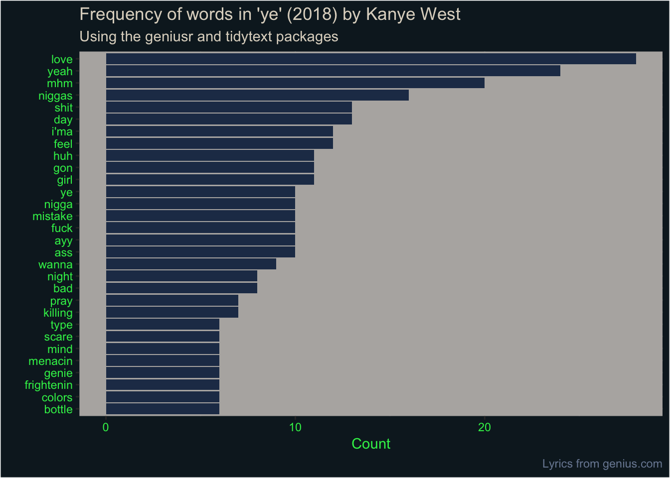
Let’s also show this as a plot. For simplicity, we’ll show only the words that appeared more than five times.
I’ve sampled seven colours from the album cover of ye, stored as hexadecimal values in a vector that’s part of the dray package. We can select from these to decorate our plot, because why not. The album cover is a Wyoming mountainscape, taken on Kanye’s own iPhone shortly before he held a listening party for the new album. Scrawled in green lettering over the image is the phrase ‘I hate being Bi-Polar it’s awesome’. (You can create your own version.)
#devtools::install_github("matt-dray/dray")
library(dray)  # for ye_cols
dray::ye_cols  # see the named colours
## mountain_blue grass_blue cloud_blue1 cloud_white cloud_grey
## "#233956" "#0e1e27" "#7a8aa2" "#dfd7c9" "#b5b2b0"
## cloud_blue2 text_green
## "#9da3ae" "#31ef56"Okay, on with the plot.
library(ggplot2)  # plots

ye_words %>%
  dplyr::count(word, sort = TRUE) %>%  # tally words
  dplyr::filter(n > 5) %>%  # more than5 occurrences
  dplyr::mutate(word = reorder(word, n)) %>%  # order by count
  ggplot2::ggplot(aes(word, n)) +
  geom_col(fill = ye_cols["mountain_blue"]) +
  labs(
    title = "Frequency of words in 'ye' (2018) by Kanye West",
    subtitle = "Using the geniusr and tidytext packages",
    x = "", y = "Count",
    caption = "Lyrics from genius.com"
  ) +
  coord_flip() +
  theme(  # apply ye theming
    plot.title = element_text(colour = ye_cols["cloud_white"]),
    plot.subtitle = element_text(colour = ye_cols["cloud_white"]),
    plot.caption = element_text(colour = ye_cols["cloud_blue1"]),
    axis.title = element_text(colour = ye_cols["text_green"]),
    axis.text = element_text(colour = ye_cols["text_green"]),
    plot.background = element_rect(fill = ye_cols["grass_blue"]),
    panel.background = element_rect(fill = ye_cols["cloud_grey"]),
    panel.grid = element_line(ye_cols["cloud_grey"])
  )
Bigrams
Extract
Tokenising by individual words is fine, but we aren’t restricted to unigrams. We can also tokenise by bigrams, which are pairs of adjacent words. For example, ‘damn croissant’ is a bigram in the sentence ‘hurry up with my damn croissaint’.
ye_bigrams <- ye_lyrics %>%
  tidytext::unnest_tokens(
    bigram,
    line,
    token = "ngrams",
    n = 2
  )
Removing stopwords is tricker than for tokenising by word. We should tokenise by bigram first, then separate the words and match them to our stopword list.
library(tidyr)  # to isolate bigram words

ye_bigrams_separated <- ye_bigrams %>%
  tidyr::separate(
    bigram,
    c("word1", "word2"),
    sep = " "
  )
Then we can filter to remove the stopwords.
ye_bigrams_filtered <- ye_bigrams_separated %>%
  dplyr::filter(
    !word1 %in% tidytext::stop_words$word,
    !word2 %in% tidytext::stop_words$word
  ) %>%
  dplyr::mutate(bigram = paste(word1, word2))
The results look a bit like this:
sample_n(ye_bigrams_filtered, 10) %>%
  dplyr::select(bigram, song_name)
## # A tibble: 10 x 2
## bigram song_name
## <chr> <chr>
## 1 bleed yeah Ghost Town
## 2 fallin dreamin Violent Crimes
## 3 premeditated murder I Thought About Killing You
## 4 gonna leave All Mine
## 5 shit halfway I Thought About Killing You
## 6 til niggas Violent Crimes
## 7 shit nigga Yikes
## 8 supermodel thick All Mine
## 9 mhm mhm I Thought About Killing You
## 10 ayy i'ma All MineCount bigrams
So let’s count the most frequent bigram occurrences, like we did for the single words.
ye_bigrams_filtered %>%
  dplyr::mutate(bigram = as.factor(bigram)) %>%
  dplyr::count(bigram, sort = TRUE) %>%
  DT::datatable(
    options = list(
      autoWidth = TRUE,
      pageLength = 10
    )
  )
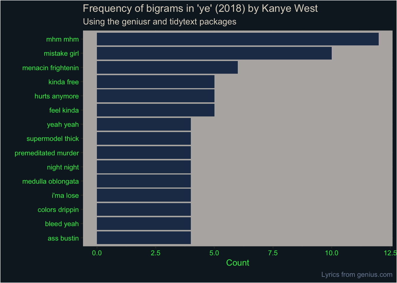
And once again we can plot this with our ye theming.
ye_bigrams_filtered %>%
  dplyr::count(bigram, sort = TRUE) %>%
  dplyr::filter(n > 3) %>%
  dplyr::mutate(bigram = reorder(bigram, n)) %>%
  ggplot2::ggplot(aes(bigram, n)) +
  geom_col(fill = ye_cols["mountain_blue"]) +
  labs(
    title = "Frequency of bigrams in 'ye' (2018) by Kanye West",
    subtitle = "Using the geniusr and tidytext packages",
    x = "", y = "Count",
    caption = "Lyrics from genius.com"
  ) +
  coord_flip() +
  theme(  # apply ye theming
    plot.title = element_text(colour = ye_cols["cloud_white"]),
    plot.subtitle = element_text(colour = ye_cols["cloud_white"]),
    plot.caption = element_text(colour = ye_cols["cloud_blue1"]),
    axis.title = element_text(colour = ye_cols["text_green"]),
    axis.text = element_text(colour = ye_cols["text_green"]),
    plot.background = element_rect(fill = ye_cols["grass_blue"]),
    panel.background = element_rect(fill = ye_cols["cloud_grey"]),
    panel.grid = element_line(ye_cols["cloud_grey"])
  )
What did we learn?
It’s difficult to get a deep insight from looking at individual words from a 24-minute, seven-song album. You might argue that looking for deep insight from Kanye West’s lyrics is a fool’s errand anyway.
Despite this, ‘love’ and ‘feel’ were in the top 10, which might indicate Kanye expressing his feelings. ‘Bad’, ‘mistake’ and ‘pray’ were also repeated a bunch of times, which might also indicate what’s on Ye’s mind.
Most of the other most common words should probably have been removed as stop words but weren’t in our stop-word dictionary (e.g. ‘yeah’, ‘mhm’, ‘i’ma’, ‘gon’, ‘ayy’, ‘wanna’). Perhaps unsurprisingly, the flexibility of ‘shit’ and ‘fuck’ means they’re pretty high up the list.
We’ve seen how simple it is to use the geniusr functions search_artist(), get_artist_meta(), get_artist_songs(), get_songs_meta() and scrape_lyrics_url() in conjunction with purrr, followed by some tidytext.
The next step might be to look at Ye’s entire back catalogue and see how his lyrics have changed over time and how they compare to ye in particular.
Obviously I only made this post for the ‘tid-ye-text’ pun, so take it or leave it.

I’m sorry, I’mma let you finish, but this sessionInfo() was the best sessionInfo() of all time
sessionInfo()## R version 3.4.3 (2017-11-30)
## Platform: x86_64-apple-darwin15.6.0 (64-bit)
## Running under: macOS High Sierra 10.13.4
##
## Matrix products: default
## BLAS: /Library/Frameworks/R.framework/Versions/3.4/Resources/lib/libRblas.0.dylib
## LAPACK: /Library/Frameworks/R.framework/Versions/3.4/Resources/lib/libRlapack.dylib
##
## locale:
## [1] en_GB.UTF-8/en_GB.UTF-8/en_GB.UTF-8/C/en_GB.UTF-8/en_GB.UTF-8
##
## attached base packages:
## [1] methods stats graphics grDevices utils datasets base
##
## other attached packages:
## [1] tidyr_0.7.2 ggplot2_2.2.1.9000 dray_0.0.0.9000
## [4] DT_0.4.5 tidytext_0.1.4 bindrcpp_0.2
## [7] purrr_0.2.4 knitr_1.18 dplyr_0.7.4
## [10] geniusr_1.0.0.9000 emo_0.0.0.9000
##
## loaded via a namespace (and not attached):
## [1] httr_1.3.1 jsonlite_1.5 shiny_1.1.0
## [4] assertthat_0.2.0 highr_0.6 selectr_0.3-1
## [7] yaml_2.1.18 slam_0.1-42 pillar_1.2.1
## [10] backports_1.1.1 lattice_0.20-35 glue_1.2.0
## [13] digest_0.6.15 RColorBrewer_1.1-2 promises_1.0.1
## [16] rvest_0.3.2 colorspace_1.3-2 htmltools_0.3.6
## [19] httpuv_1.4.3 Matrix_1.2-12 plyr_1.8.4
## [22] psych_1.7.8 XML_3.98-1.9 pkgconfig_2.0.1
## [25] broom_0.4.2 bookdown_0.5 xtable_1.8-2
## [28] scales_0.5.0.9000 later_0.7.2 tibble_1.4.2
## [31] withr_2.1.2 lazyeval_0.2.1 cli_1.0.0
## [34] mnormt_1.5-5 magrittr_1.5 crayon_1.3.4
## [37] mime_0.5 evaluate_0.10.1 tokenizers_0.1.4
## [40] janeaustenr_0.1.5 nlme_3.1-131 SnowballC_0.5.1
## [43] xml2_1.2.0 foreign_0.8-69 blogdown_0.1
## [46] tools_3.4.3 stringr_1.3.0 munsell_0.4.3
## [49] plotrix_3.7-2 compiler_3.4.3 rlang_0.2.1
## [52] grid_3.4.3 htmlwidgets_1.0 crosstalk_1.0.1
## [55] labeling_0.3 rmarkdown_1.6 gtable_0.2.0
## [58] curl_3.0 reshape2_1.4.3 R6_2.2.2
## [61] lubridate_1.7.2 utf8_1.1.3 bindr_0.1
## [64] rprojroot_1.2 stringi_1.1.7 parallel_3.4.3
## [67] Rcpp_0.12.17 wordcloud_2.5 tidyselect_0.2.3This is not a review of the album. There’s plenty of those already.↩
This is also not a commentary on his many controversies.↩
An API is an ‘Application Programme Interface’, which is a fancy way of saying ‘computers talking to computers’.↩
Note that there’s also a
geniusRpackage, which has a very similar name, but has to be installed from GitHub rather than CRAN.↩