‘Walrus rainbow vomit’ is a sentence I’d never thought I’d type (via Giphy)

Note

I later learnt about {colorfindr} by David Zumbach, which can extract colours from images, provide composition details and generate palettes. Check it out.

tl;dr

I used the {magick} package in R to map an image’s colours to their nearest match from a simplified palette, then quantified how much of the image was covered by each colour in that palette.

Colour search

As a side project at work, we wanted users to be able to search images of artwork by their prevalence of colours from a small simple palette (red, blue, yellow, etc).

Lots of online services let you sort images by colour. Our inspiration included:

Art of the possible

What might be a relatively simple and straightforward way to do this in R?

By ‘simple’ I mean we don’t want to do any hard work. We don’t want to consider any colour theory¹ and we want to stick to simple, easily-named colours like ‘green’.²

So, we want to do the following:

Read in an image
Prepare a set of ‘simple colours’
Map the simple colours to the image
Quantify the colours

It’s a kind of ImageMagick

The {magick} R package is an implementation of ImageMagick, an open-source software suite whose emphasis is image manipulation from the command line. The flexibility of {magick} can be seen in its vignette.

The package was created and is maintained by Jeroen Ooms, a software engineer and postdoc at rOpenSci, a collective that seeks to develop tools for open and reproducible research.

rOpenSci hosted a workshop from Ooms about working with images in R and the presentation slides caught my attention. I’ve used some of Jeroen’s code below.

Code

First we need to load our packages. {magick} is available from CRAN.

# All available from CRAN with install.packages()
library(dplyr)   # tidy data manipulation
library(tibble)  # tidy tables
library(magick)  # image manipulation

Read a test image

I’ve chosen a colourful image to use for our test case: it’s a picture of a bunch of Lego Duplo bricks.³

We’ll use image_read() to read the JPEG as an object of class ‘magick’ and then image_scale() to reduce the image size and save some space.

Printing the image also gives us some details of format, dimensions, etc.

# Path to the image
duplo_path <- "https://upload.wikimedia.org/wikipedia/commons/thumb/a/ac/Lego_dublo_arto_alanenpaa_2.JPG/2560px-Lego_dublo_arto_alanenpaa_2.JPG"

# Read as magick object and resize
duplo <- image_read(duplo_path) %>%
  image_scale(geometry = c("x600"))

print(duplo)

## # A tibble: 1 x 7
##   format width height colorspace matte filesize density
##   <chr>  <int>  <int> <chr>      <lgl>    <int> <chr>  
## 1 JPEG     900    600 sRGB       FALSE        0 72x72

Prepare simple colours

We’ll map a set of simple colours to the test image. This means that the colours from the test image will be replaced by the ‘closest’ colour from our simple set.

One way to do this is to define our simple colour set and create an image from them. In this case I’m taking just six colours.

# Generate named vector of 'simple' colours
cols_vec <- setNames(
  c("#000000", "#0000ff", "#008000", "#ff0000", "#ffffff", "#ffff00"),
  c("black", "blue", "green", "red", "white", "yellow")
)

Then we can plot squares of these colours, using image_graph() to read them as magick-class objects.⁴ My method here is not the most efficient, but you can see the output is an image that contains our six colours.

Click for code

# For each vector element (colour) create a square of that colour
for (i in seq_along(cols_vec)) {
  fig_name <- paste0(names(cols_vec)[i], "_square")  # create object name
  assign(
    fig_name,  # set name
    image_graph(width = 100, height = 100, res = 300)  # create magick object
  )
  par(mar = rep(0, 4))  # set plot margins
  plot.new()  # new graphics frame
  rect(0, 0, 1, 1, col = cols_vec[i], border = cols_vec[i])  # build rectangle
  assign(fig_name, magick::image_crop(get(fig_name), "50x50+10+10")) # crop
  dev.off()  # shut down plotting device
  rm(i, fig_name)  # clear up
}

# Generate names of the coloured square objects
col_square <- paste0(names(cols_vec), "_square")

# Combine magick objects (coloured squares)
simple_cols <- image_append(c(
  get(col_square[1]), get(col_square[2]), get(col_square[3]),
  get(col_square[4]), get(col_square[5]), get(col_square[6])
))

print(simple_cols)

## # A tibble: 1 x 7
##   format width height colorspace matte filesize density
##   <chr>  <int>  <int> <chr>      <lgl>    <int> <chr>  
## 1 PNG      300     50 sRGB       TRUE         0 72x72

Map to the image

Now we can apply the simple colour set to the test image using image_map().

# Map the simple colours to the image
duplo_mapped <- image_map(
  image = duplo,  # original image
  map = simple_cols  # colours to map on
)

And we can use image_animate() to see the difference between the two.

# Display the original and simplified images side by side
image_animate(c(duplo, duplo_mapped), fps = 1)

Great. You can see where the original colours have been replaced by the ‘closest’ simple colours.

Note in particular where the more reflective surfaces are mapped to white than the actual brick colour.

This is okay: the brick may be blue, but we’ve only defined one shade of blue. If a particular shade is closer to white, then so be it.

Quantify the colours

Now we can take this mapped image and quantify how much of the image belongs to each colour. Imagine we’ve broken the image into pixels and then we’re counting how many belng to each of our six colours.

# Function to count the colours (adapted from Jeroen Ooms)
count_colors <- function(image) {
  data <- image_data(image) %>%
    apply(2:3, paste, collapse = "") %>% 
    as.vector %>% table() %>%  as.data.frame() %>% 
    setNames(c("hex", "freq"))
  data$hex <- paste("#", data$hex, sep="")
  return(data)
}

# Dataframe of dominant colours 
duplo_col_freq <- duplo_mapped %>%
  count_colors() %>%
  left_join(
    enframe(cols_vec) %>% rename(hex = value),
    by = "hex"
  ) %>% 
  arrange(desc(freq)) %>% 
  mutate(percent = 100*round((freq/sum(freq)), 3)) %>% 
  select(
    `Colour name` = name, Hexadecimal = hex,
    `Frequency of colour` = freq, `Percent of image` = percent
  )

duplo_mapped  # see mapped image again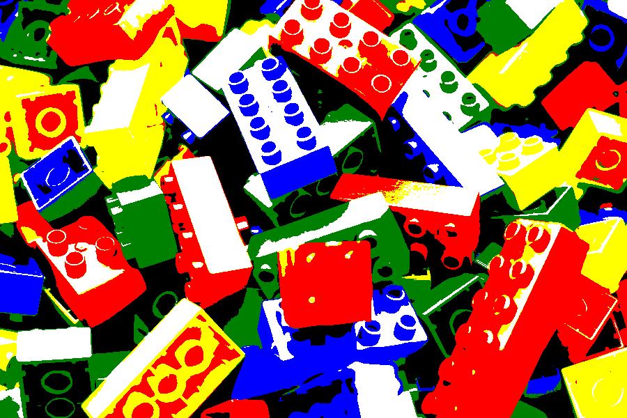

knitr::kable(duplo_col_freq)  # quantify colour

Colour name	Hexadecimal	Frequency of colour	Percent of image
red	#ff0000	132134	24.5
white	#ffffff	107847	20.0
black	#000000	103641	19.2
yellow	#ffff00	79751	14.8
green	#008000	64867	12.0
blue	#0000ff	51760	9.6

So red makes up almost a quarter of the image, with white and black just behind. This makes sense: many of the bricks are red and much of the shadow areas of yellow bricks were rendered as red, while black and white make up many of the other shadows and reflective surfaces.

And so we must p-art

So, you can map a simple colour set to an image with {magick} and then quantify how much of the image is covered by that simple set.

Of course, there are many possibilities beyond what’s been achieved here. For example, you could create a tool where the user chooses a colour and images are returned in order of dominance for that colour. You could also write this all into a function that takes a folder of images and returns the percentage of each colour in each image.

Below are some additional examples of the approach taken in this post.

Reef fish

Click for details

Image by Richard L Pyle from Wikimedia Commons, CC0 1.0.

reef_path <- "https://upload.wikimedia.org/wikipedia/commons/0/05/100%25_reef-fish_Endemism_at_90_m_off_Kure_Atoll.jpg"

reef <- image_read(reef_path) %>%
  image_scale(geometry = c("x600"))

reef_mapped <- image_map(
  image = reef,  # original image
  map = simple_cols  # colours to map on
)

reef_col_freq <- reef_mapped %>%
  count_colors() %>%
  left_join(
    enframe(cols_vec) %>% rename(hex = value),
    by = "hex"
  ) %>% 
  arrange(desc(freq)) %>% 
  mutate(percent = 100*round((freq/sum(freq)), 3)) %>% 
  select(
    `Colour name` = name, Hexadecimal = hex,
    `Frequency of colour` = freq, `Percent of image` = percent
  )

reef_animate <- image_animate(c(reef, reef_mapped), fps = 1)

Colour name	Hexadecimal	Frequency of colour	Percent of image
blue	#0000ff	317133	49.5
black	#000000	214647	33.5
green	#008000	76245	11.9
yellow	#ffff00	13296	2.1
red	#ff0000	10079	1.6
white	#ffffff	8800	1.4

Hong Kong lights

Click for details

Image by Daniel Case from Wikimedia Commons, CC BY-SA 3.0

neon_path <- "https://upload.wikimedia.org/wikipedia/commons/thumb/b/b0/Neon_lights%2C_Nathan_Road%2C_Hong_Kong.jpg/900px-Neon_lights%2C_Nathan_Road%2C_Hong_Kong.jpg"

neon <- image_read(neon_path) %>%
  image_scale(geometry = c("x600"))

neon_mapped <- image_map(
  image = neon,  # original image
  map = simple_cols  # colours to map on
)

neon_col_freq <- neon_mapped %>%
  count_colors() %>%
  left_join(
    enframe(cols_vec) %>% rename(hex = value),
    by = "hex"
  ) %>% 
  arrange(desc(freq)) %>% 
  mutate(percent = 100*round((freq/sum(freq)), 3)) %>% 
  select(
    `Colour name` = name, Hexadecimal = hex,
    `Frequency of colour` = freq, `Percent of image` = percent
  )

neon_animate <- image_animate(c(neon, neon_mapped), fps = 1)

Colour name	Hexadecimal	Frequency of colour	Percent of image
black	#000000	191565	71.0
green	#008000	23134	8.6
blue	#0000ff	18455	6.8
red	#ff0000	17551	6.5
yellow	#ffff00	10874	4.0
white	#ffffff	8421	3.1

Ladybird

Click for details

Image by Elena Andreeva from Wikimedia Commons, CC0 1.0.

lbird_path <- "https://upload.wikimedia.org/wikipedia/commons/d/d5/Erysimum_Cheiranthoides_%28215134987%29.jpeg"

lbird <- image_read(lbird_path) %>%
  image_scale(geometry = c("x600"))

lbird_mapped <- image_map(
  image = lbird,  # original image
  map = simple_cols  # colours to map on
)

lbird_col_freq <- lbird_mapped %>%
  count_colors() %>%
  left_join(
    enframe(cols_vec) %>% rename(hex = value),
    by = "hex"
  ) %>% 
  arrange(desc(freq)) %>% 
  mutate(percent = 100*round((freq/sum(freq)), 3)) %>% 
  select(
    `Colour name` = name, Hexadecimal = hex,
    `Frequency of colour` = freq, `Percent of image` = percent
  )

lbird_animate <- image_animate(c(lbird, lbird_mapped), fps = 1)

Colour name	Hexadecimal	Frequency of colour	Percent of image
white	#ffffff	300366	54.2
blue	#0000ff	117361	21.2
yellow	#ffff00	100809	18.2
green	#008000	27647	5.0
black	#000000	5305	1.0
red	#ff0000	2312	0.4

Session info

## [1] "Last updated 2021-02-08"

## ─ Session info ───────────────────────────────────────────────────────────────
##  setting  value                       
##  version  R version 3.6.3 (2020-02-29)
##  os       macOS  10.16                
##  system   x86_64, darwin15.6.0        
##  ui       X11                         
##  language (EN)                        
##  collate  en_GB.UTF-8                 
##  ctype    en_GB.UTF-8                 
##  tz       Europe/London               
##  date     2021-02-08                  
## 
## ─ Packages ───────────────────────────────────────────────────────────────────
##  package     * version date       lib source                            
##  assertthat    0.2.1   2019-03-21 [1] CRAN (R 3.6.0)                    
##  blogdown      0.12    2019-05-01 [1] CRAN (R 3.6.0)                    
##  bookdown      0.10    2019-05-10 [1] CRAN (R 3.6.0)                    
##  cli           2.3.0   2021-01-31 [1] CRAN (R 3.6.2)                    
##  crayon        1.4.0   2021-01-30 [1] CRAN (R 3.6.2)                    
##  curl          4.3     2019-12-02 [1] CRAN (R 3.6.0)                    
##  digest        0.6.27  2020-10-24 [1] CRAN (R 3.6.2)                    
##  dplyr       * 0.8.3   2019-07-04 [1] CRAN (R 3.6.0)                    
##  ellipsis      0.3.1   2020-05-15 [1] CRAN (R 3.6.2)                    
##  evaluate      0.14    2019-05-28 [1] CRAN (R 3.6.0)                    
##  fansi         0.4.2   2021-01-15 [1] CRAN (R 3.6.2)                    
##  glue          1.4.2   2020-08-27 [1] CRAN (R 3.6.2)                    
##  highr         0.8     2019-03-20 [1] CRAN (R 3.6.0)                    
##  htmltools     0.4.0   2019-10-04 [1] CRAN (R 3.6.0)                    
##  icon          0.1.0   2019-10-09 [1] Github (ropenscilabs/icon@a5bc1cc)
##  knitr         1.31    2021-01-27 [1] CRAN (R 3.6.2)                    
##  lifecycle     0.2.0   2020-03-06 [1] CRAN (R 3.6.0)                    
##  magick      * 2.2     2019-08-26 [1] CRAN (R 3.6.0)                    
##  magrittr      2.0.1   2020-11-17 [1] CRAN (R 3.6.2)                    
##  pillar        1.4.7   2020-11-20 [1] CRAN (R 3.6.2)                    
##  pkgconfig     2.0.3   2019-09-22 [1] CRAN (R 3.6.0)                    
##  png           0.1-7   2013-12-03 [1] CRAN (R 3.6.0)                    
##  purrr         0.3.4   2020-04-17 [1] CRAN (R 3.6.2)                    
##  R6            2.5.0   2020-10-28 [1] CRAN (R 3.6.2)                    
##  Rcpp          1.0.3   2019-11-08 [1] CRAN (R 3.6.0)                    
##  rlang         0.4.10  2020-12-30 [1] CRAN (R 3.6.2)                    
##  rmarkdown     2.0     2019-12-12 [1] CRAN (R 3.6.0)                    
##  sessioninfo   1.1.1   2018-11-05 [1] CRAN (R 3.6.0)                    
##  stringi       1.5.3   2020-09-09 [1] CRAN (R 3.6.2)                    
##  stringr       1.4.0   2019-02-10 [1] CRAN (R 3.6.0)                    
##  tibble      * 3.0.6   2021-01-29 [1] CRAN (R 3.6.2)                    
##  tidyselect    0.2.5   2018-10-11 [1] CRAN (R 3.6.0)                    
##  utf8          1.1.4   2018-05-24 [1] CRAN (R 3.6.0)                    
##  vctrs         0.3.6   2020-12-17 [1] CRAN (R 3.6.2)                    
##  withr         2.4.1   2021-01-26 [1] CRAN (R 3.6.2)                    
##  xfun          0.20    2021-01-06 [1] CRAN (R 3.6.2)                    
##  yaml          2.2.1   2020-02-01 [1] CRAN (R 3.6.0)                    
## 
## [1] /Library/Frameworks/R.framework/Versions/3.6/Resources/library

Just as well, because I’m colourblind.↩︎
There are five named versions of olive drab in R’s named palette.↩︎
Photo by Arto Alanenpää, CC0-BY-4.0 from Wikimedia Creative Commons.↩︎
Artefacts introduced during compression of PNGs and JPGs might mean that your set of six colours ends up being more than six. It’s preferable to generate our colour set within R, inside image_graph(), so that we have only our six defined colours.↩︎

Quantify colour by {magick}

tl;dr

Colour search

Art of the possible

It’s a kind of ImageMagick

Code

Read a test image

Prepare simple colours

Map to the image

Quantify the colours

And so we must p-art

Reef fish

Hong Kong lights

Ladybird