tl;dr

You can convert a line drawing to datapoints with a sprinkle of {magick}.

Ape escape

Have you seen that video where you’re so focused on counting basketball passes that you fail to see the gorilla moving across the screen?

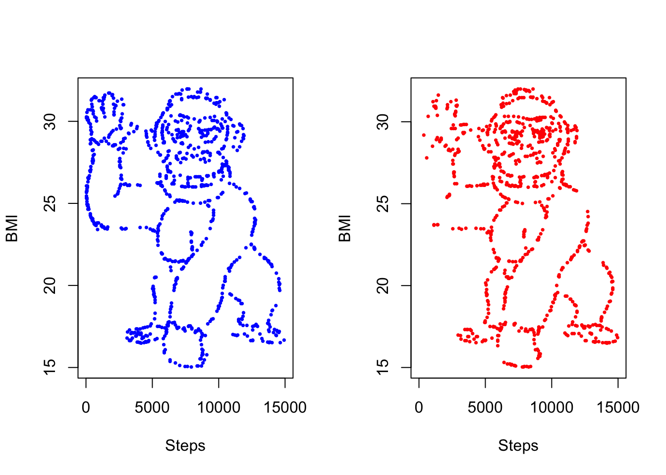
This kind of selective attention was studied by two researchers, Yanai and Lercher, who provided subjects with a dataset that looked like a gorilla when plotted. The gorilla was found less often if the subjects were also given a hypothesis to investigate.

The study got some attention on Twitter last week. As a result, Isabella Velásquez wrote a great blogpost where she recreated the dataset using R and Python in tandem via the {reticulate} package.

I had a go at creating the dataset with base R and the excellent {magick} package for image manipulation.

Point it out

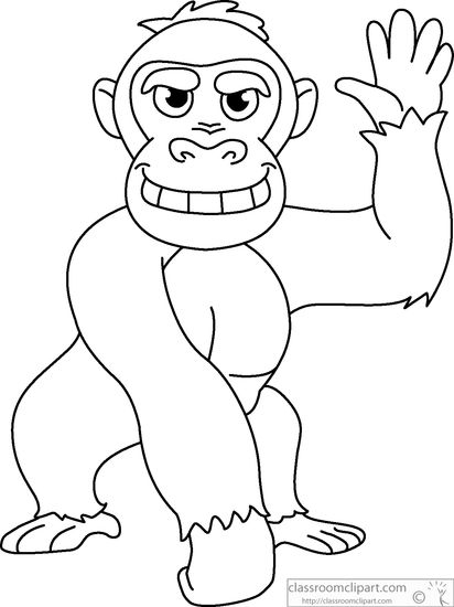
The jpeg image file used in the original paper can be downloaded from classroomclipart.com to a temporary location on your machine.

download.file(
  paste0(
    "https://classroomclipart.com/images/gallery/",
    "Clipart/Black_and_White_Clipart/Animals/",
    "gorilla-waving-cartoon-black-white-outline-clipart-914.jpg" 
  ),
  tempfile(fileext = ".jpg")
)

We can read the file into R with {magick}.

img <- 
  list.files(tempdir(), pattern = ".jpg$", full.names = TRUE) |>
  magick::image_read()

img

With other {magick} functions we can:

• reduce to two distinct colours only (i.e. for the lines and background), which makes it easier to filter the data later
• convert from an image to point data

go <- img |>
  magick::image_quantize(2) |>  # colour reduction
  magick::image_raster() |>     # as x-y data
  as.data.frame()

head(go)

##   x y       col
## 1 1 1 #fefefeff
## 2 2 1 #fefefeff
## 3 3 1 #fefefeff
## 4 4 1 #fefefeff
## 5 5 1 #fefefeff
## 6 6 1 #fefefeff

And to prove we only have two colours (off-white for the background, grey for the lines):

unique(go$col)

## [1] "#fefefeff" "#555555ff"

Now we can:

• reverse the order of the y values so the gorilla faces the same way as in the paper
• filter to retain only the datapoints that represent lines
• rescale the x and y to create ‘Body Mass Index’ (BMI)¹ and ‘steps’ variables

go$y     <- rev(go$y)
go       <- go[go$col != "#fefefeff", ]
go$bmi   <- go$y / max(go $y) * 17 + 15
go$steps <- 15000 - go$x * 15000 / max(go$x)

head(go)

##       x   y       col bmi    steps
## 174 174 550 #555555ff  32 8665.049
## 175 175 550 #555555ff  32 8628.641
## 176 176 550 #555555ff  32 8592.233
## 196 196 550 #555555ff  32 7864.078
## 198 198 550 #555555ff  32 7791.262
## 199 199 550 #555555ff  32 7754.854

You may have noticed that the image has a watermark. We could have removed it earlier with {magick}, but can do it now by filtering out the datapoints in that corner.

go$logo <- ifelse(go$bmi < 16 & go$steps < 5500, TRUE, FALSE)
go      <- go[!go$logo, ]

This leaves us with 16865 datapoints. We can follow the original study by taking a sample and splitting the results into ‘female’ and ‘male’ groups, weighted so that the female group has higher step counts.

go_smp       <- go[sample(nrow(go), 1768), ]
go_smp$rnorm <- rnorm(nrow(go_smp), mean = 0, sd = 10)
go_smp$index <- go_smp$steps * (1 + go_smp$rnorm)
go_smp$group <- 
  ifelse(go_smp$index < median(go_smp$steps), "F", "M") |>
  as.factor()

head(go_smp[, c("bmi", "steps", "group")])

##             bmi      steps group
## 141108 21.42909 7572.81553     F
## 78949  26.09636 5643.20388     F
## 28681  29.86727 5788.83495     M
## 90859  25.20000 7026.69903     F
## 78506  26.12727 6771.84466     M
## 81986  25.88000   72.81553     F

Now finally to plot the datasets side-by-side.

par(mfrow = c(1, 2))

with(
  go_smp[go_smp$group == "F", ],
  plot(
    steps, bmi, xlim = c(0, 15000),
    pch = 16, cex = 0.5, col = "blue",
    xlab = "Steps", ylab = "BMI", 
  )
)

with(
  go_smp[go_smp$group == "M", ],
  plot(
    steps, bmi, xlim = c(0, 15000),
    pch = 16, cex = 0.5, col = "red",
    xlab = "Steps", ylab = "BMI"
  )
)

I see them!

This has been a bit overengineered and could be generalised, but it gives a gist of how you might go about converting an image to a dataframe of x and y positions.

At worst, this is a reminder not to trust researchers and to always check for unexpected gorillas.

## ─ Session info ───────────────────────────────────────────────────────────────
##  setting  value                       
##  version  R version 4.1.1 (2021-08-10)
##  os       macOS Mojave 10.14.6        
##  system   x86_64, darwin17.0          
##  ui       X11                         
##  language (EN)                        
##  collate  en_GB.UTF-8                 
##  ctype    en_GB.UTF-8                 
##  tz       Europe/London               
##  date     2021-10-05                  
## 
## ─ Packages ───────────────────────────────────────────────────────────────────
##  package     * version date       lib source        
##  blogdown      1.5     2021-09-02 [1] CRAN (R 4.1.0)
##  bookdown      0.24    2021-09-02 [1] CRAN (R 4.1.0)
##  bslib         0.3.0   2021-09-02 [1] CRAN (R 4.1.0)
##  cli           3.0.1   2021-07-17 [1] CRAN (R 4.1.0)
##  digest        0.6.28  2021-09-23 [1] CRAN (R 4.1.0)
##  evaluate      0.14    2019-05-28 [1] CRAN (R 4.1.0)
##  fastmap       1.1.0   2021-01-25 [1] CRAN (R 4.1.0)
##  highr         0.9     2021-04-16 [1] CRAN (R 4.1.0)
##  htmltools     0.5.2   2021-08-25 [1] CRAN (R 4.1.0)
##  jquerylib     0.1.4   2021-04-26 [1] CRAN (R 4.1.0)
##  jsonlite      1.7.2   2020-12-09 [1] CRAN (R 4.1.0)
##  knitr         1.34    2021-09-09 [1] CRAN (R 4.1.0)
##  magick        2.7.3   2021-08-18 [1] CRAN (R 4.1.0)
##  magrittr      2.0.1   2020-11-17 [1] CRAN (R 4.1.0)
##  R6            2.5.1   2021-08-19 [1] CRAN (R 4.1.0)
##  Rcpp          1.0.7   2021-07-07 [1] CRAN (R 4.1.0)
##  rlang         0.4.11  2021-04-30 [1] CRAN (R 4.1.0)
##  rmarkdown     2.11    2021-09-14 [1] CRAN (R 4.1.0)
##  rstudioapi    0.13    2020-11-12 [1] CRAN (R 4.1.0)
##  sass          0.4.0   2021-05-12 [1] CRAN (R 4.1.0)
##  sessioninfo   1.1.1   2018-11-05 [1] CRAN (R 4.1.0)
##  stringi       1.7.4   2021-08-25 [1] CRAN (R 4.1.0)
##  stringr       1.4.0   2019-02-10 [1] CRAN (R 4.1.0)
##  withr         2.4.2   2021-04-18 [1] CRAN (R 4.1.0)
##  xfun          0.26    2021-09-14 [1] CRAN (R 4.1.0)
##  yaml          2.2.1   2020-02-01 [1] CRAN (R 4.1.0)
## 
## [1] /Users/matt.dray/Library/R/x86_64/4.1/library
## [2] /Library/Frameworks/R.framework/Versions/4.1/Resources/library